Aeropendulum (theory)
Analysis of a damped driven pendulum with a step torque input starting at \(t = 0\), including:
Equations of motion
Equilibrium point shift
Natural frequency change
Time-dependent solution with initial conditions:
\[\theta(0) = 0, \quad \dot{\theta}(0) = 0\]
System Description
Mass: \(m\)
Length: \(L\)
Damping coefficient: \(b\) (viscous damping torque \(= b \dot{\theta}\))
Gravitational torque: \(\tau_g = -mgL \sin\theta\)
Driving torque: \(\tau_d(t) = \tau_0 \cdot u(t)\) (step function)
Using Newton’s 2nd law for rotation:
where \(I = mL^2\) is the moment of inertia.
Linearized Equation of Motion
For small angles (\(\theta \ll 1\)), we linearize \(\sin\theta \approx \theta\). Then:
Dividing through by \(mL^2\):
Define:
\(\omega_0 = \sqrt{\frac{g}{L}}\) (undamped natural frequency)
\(\zeta = \frac{b}{2mL^2 \omega_0}\) (damping ratio)
\(A = \frac{\tau_0}{mL^2}\) (normalized torque)
So the linear equation is:
Equilibrium Position Shift
Set derivatives to zero in the steady-state:
This is the new equilibrium position under constant torque.
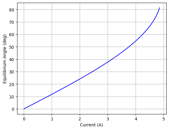
[1]:
import numpy as np
import matplotlib.pyplot as plt

# Physical constants
g = 9.81       # gravity (m/s^2)
L = 0.1        # length of pendulum (m)
m = 0.1        # mass (kg)

km=0.02
I=np.linspace(0,6, 100)

tetaeq=np.asin(I*km/(m*g*L))*180/3.14
plt.plot(I, tetaeq, label='eq', color='blue')
plt.xlabel("Current (A)")
plt.ylabel("Equilibrium Angle (deg)")
plt.grid(True)
C:\Users\Utilizador\AppData\Local\Temp\ipykernel_15004\749860262.py:12: RuntimeWarning: invalid value encountered in arcsin
  tetaeq=np.asin(I*km/(m*g*L))*180/3.14
Time-Dependent Solution
This is a standard second-order linear ODE with step forcing. The general solution is:
Particular solution:
Homogeneous solution:
Solve:
The solution depends on damping regime.
Case: Underdamped (\(\zeta < 1\))
Let:
Then:
This satisfies:
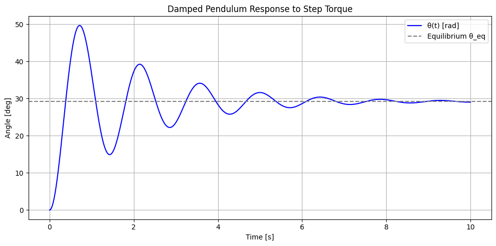
[15]:
import numpy as np
import matplotlib.pyplot as plt

# Physical parameters
m = 0.2          # mass (kg)
L = 0.5          # pendulum length (m)
b = 0.05          # damping coefficient (N*m*s)
g = 9.81         # gravity (m/s^2)

# Torque input (step change)
tau_0 = 0.5      # torque applied after t=0 (N*m)

# Initial conditions
theta_0 = 0.0    # initial angle (rad)
omega_0 = 0.0    # initial angular velocity (rad/s)

# Derived parameters
I = m * L**2
omega_n = np.sqrt(g / L)
zeta = b / (2 * I * omega_n)
omega_d = omega_n * np.sqrt(1 - zeta**2)
theta_eq = tau_0 / (m * g * L)   # new equilibrium position

# Time vector
t = np.linspace(0, 10, 1000)  # 10 seconds, 1000 points

# Coefficients A and B from general solution
A = theta_0 - theta_eq
B = (omega_0 + zeta * omega_n * A) / omega_d

# Analytical solution
theta_t = theta_eq + np.exp(-zeta * omega_n * t) * (A * np.cos(omega_d * t) + B * np.sin(omega_d * t))

#Conversion
rad2deg=180/3.14

# Plotting
plt.figure(figsize=(10, 5))
plt.plot(t, theta_t*rad2deg, label='θ(t) [rad]', color='blue')
plt.axhline(theta_eq*rad2deg, color='gray', linestyle='--', label='Equilibrium θ_eq')
plt.title('Damped Pendulum Response to Step Torque')
plt.xlabel('Time [s]')
plt.ylabel('Angle [deg]')
plt.grid(True)
plt.legend()
plt.tight_layout()
plt.show()